suppose we have a set of measurements $y_1,y_2,\ldots,y_N$ that we would like to compare to the model
\begin{equation}
f_n = a + b \cos\left(\frac{2\pi n}{N} - \delta\right)
\label{eq:c}
\end{equation}
where $a,b,\delta$ are all (real) parameters.
In particular we are interested in the ratio $b/a \equiv r$ which we will refer as $A$.
The measurements are made in the presence of noise so that we can expect a mean (i.e. expectation) value
$$
\ev{y_n} = f_n
$$
but repeated measurements at fixed $n$ are liable to differ by some amount $\delta y$, we which we assume to be gaussian distributed and independent of $n$.
We also assume distinct measurements are independents which tells us that
\begin{equation}
\ev{y_n y_{n'}} = f_n f_{n'} + \delta y^2 \delta_{nn'}
\label{eq:ind}
\end{equation}
How can we use our measurements to estimate $A$ and the uncertainty $\delta A$ in our estimate due to $\delta y$?
Well math is how we're going to do it.
The first thing we will note is that our model (equation \eqref{eq:c}) can be rewritten in the form
\begin{equation}
f_n = \sum_{n=1}^N c_n e^{i 2\pi n / N}
\label{eq:d}
\end{equation}
where $c_N = a \equiv c_o$, $c_1 = c^*_{N-1} = \frac{1}{2} b e^{-i\delta}$, and $c_n = 0$ otherwise.
Our ratio of interest $R$ can be written in terms of the $c_n$ as $2 |c_1|/c_o \equiv 2 R$.
Equation \eqref{eq:d} is the discrete fourier transform of a set of coefficients $c_1,c_2,\ldots,c_N$.
We can define estimators $\hat{c}_n$ for the $c_n$ via the inverse transform
\begin{equation}
\hat{c}_n \equiv \frac{1}{N}\sum_m^N y_m e^{- i 2 \pi m / N}
\label{eq:idft}
\end{equation}
These estimators turn out to be unbiased.
To see this we use the relation1
\begin{equation}
\sum_{n=1}^N e^{i 2 \pi m n / N} = N \delta_{m0}
\label{eq:a}
\end{equation}
where $m=0,1,\ldots,N-1$ and verify that the expectation value $\ev{\hat{c}_m}$ yields
\begin{align*}
\ev{\hat{c}_n} = &
\frac{1}{N} \sum_{m=1}^N e^{-i 2 \pi m n / N}\ev{y_m}
\\ = &
\frac{1}{N} \sum_{m=1}^N e^{-i 2 \pi m n / N} f_m
\\ = &
\frac{1}{N} \sum_{m=1}^N e^{-i 2 \pi m n / N} \sum{n'=1}^N c_{n'}e^{i 2 \pi n n' / N}
\\ = &
\frac{1}{N} \sum_{n'=1}^N c_{n'} \left(\sum_{m=1}^N e^{i 2 \pi m (n'-n) / N}\right)
\\ = &
\frac{1}{N} \sum_{n'=1}^N c_{n'} N \delta_{nn'}
\\ = &
c_n
\end{align*}
It also turns out that the $\hat{c}_n$ are statistically independent and have equal variances.
To see this we inspect the (complex) covariance matrix $\sigma^c_{n n'} \equiv \ev{\hat{c}_n^*\hat{c}_{n'}} - \ev{\hat{c}_n^*}\ev{\hat{c}_{n'}} = \ev{\hat{c}_n^*\hat{c}_{n'}} - c_n^*c_{n'}$ and see that
\begin{align}
\sigma^c_{n n'} = &
\frac{1}{N^2} \sum_{m,m'=1}^N e^{i 2\pi \left( m' n' - m n \right) / N} \ev{y_{m'} y_m} - c_n^*c_{n'}
\\ = &
\frac{1}{N^2} \sum_{m,m'=1}^N e^{i 2\pi \left( m' n' - m n \right) / N} \left( f_{m'} f^*_m + \delta y^2 \delta_{m'm} \right) - c_n^*c_{n'}
\\ = &
c_n^* c_{n'} + \frac{\delta y^2}{N^2} \sum_{m=1}^N e^{i 2 \pi m \left( n' - n \right) / N} - c_n^*c_{n'}
\\ = &
\frac{\delta y^2}{N^2} \sum_{m=1}^N e^{i 2 \pi m \left( n' - n \right) / N}
\\ = &
\delta \tilde{y}^2 \delta_{n n'}
\label{eq:cov}
\end{align}
where $\delta \tilde{y} \equiv \delta y / \sqrt{N}$.
We now have the main ingredients to determine the mean and variance of $\hat{R} = \sqrt{c_1 c_1^*}/c_o$. For the mean $\ev{\hat{R}}$ we find
$$
\ev{\hat{R}} =
\ev{\frac{\sqrt{\hat{c}_1^* \hat{c}_1}}{\hat{c}_o}} =
\ev{\sqrt{\hat{c}_1^* \hat{c}_1}} \ev{\frac{1}{\hat{c}_o}}
$$
by the statistical independence of the $\hat{c}_n$.
To make further progress we will use the taylor expansion for expectation values
$$
\ev{f(\hat{x})} \approx f \left( \ev{\hat{x}} \right) + \frac{1}{2} f''\left(\ev{\hat{x}}\right) \text{var}\left(\hat{x}\right)
$$
which applies so long as the distribution for $\hat{x}$ is sharply peaked compared to the variation in $f$.
Applying this for $f(\hat{x}) = \sqrt{\hat{x}}$ and $\hat{x} = |c_1|^2$ we find
$$
\ev{\sqrt{|\hat{c}_1|^2}} \approx |c_1|^2 \sqrt{1 + z_1^2} \left( 1 - \frac{1}{8} \frac{\text{var}\left(|c_1|^2\right)}{|c_1|^4 \left( 1 + z_1^2 \right)^2} \right)
$$
Where we have introduced the definition $z_n \equiv \delta \tilde{y} / |c_n|$.
It remains to compute $\text{var}\left(|\hat{c}_1|^2\right) = \ev{|\hat{c}_1|^4} - \ev{|\hat{c}_1|^2}^2$.
We already know that
$$
\ev{|\hat{c}_1|^2} = |c_1|^2 \left( 1 + z_1^2 \right)
$$
So we would like to compute $\ev{|c_1|^4}$.
By plugging in definitions we find
\begin{align*}
\ev{|c_1|^4} = &
\frac{1}{N^4} \sum_{a,b,c,d=1}^N e^{i2\pi \left( a - b + c - d \right) / N} \ev{y_a y_b y_c y_d}
\\ = &
\frac{1}{N^4} \sum_{a,b,c,d=1}^N e^{i2\pi \left( a - b + c - d \right) / N} \\
\langle & \left( \sum_{\alpha=1}^N e^{i2\pi \alpha a / N} c_a + \hat{\varepsilon}_a \right) \\
& \left( \sum_{\beta=1}^N e^{i2\pi \beta b / N} c_b + \hat{\varepsilon}_b \right) \\
& \left( \sum_{\gamma=1}^N e^{i2\pi \gamma c / N} c_c + \hat{\varepsilon}_c \right) \\
& \left( \sum_{\delta=1}^N e^{i2\pi \delta d / N} c_d + \hat{\varepsilon}_d \right) \rangle
\end{align*}
where the $\hat{\varepsilon}_i$ are independent gaussian random variables with mean zero and variance of $\delta y^2$.
The expectation value evidently contains a sum of terms, each term a product of terms obtained by selecting either the exponential sum or the $\hat{\varepsilon}_i$ from each parentheses.
The term containing all four exponential sums will reduce to $|c_1|^4$.
All terms containing an odd number of the $\hat{\varepsilon}_i$ will vanish by virtue of their zero mean.
Their are six terms containing pairs $\ev{\hat{\varepsilon}_i \hat{\varepsilon}_j}$, e.g.
$$
\left( \sum_{\alpha=1}^N e^{i2\pi \alpha a / N} c_a \right) \left( \sum_{\beta=1}^N e^{i2\pi \beta b / N} c_b \right) \ev{\hat{\varepsilon}_c \hat{\varepsilon}_d}
$$
Via equation \eqref{eq:a} and the relation $\ev{\hat{\varepsilon}_i \hat{\varepsilon}_j} = \delta y^2 \delta_{ij}$ we the particular term above contributes to $\ev{|\hat{c}_1|^4}$ as
$$
|c_1|^2 \frac{\delta y^2}{N^2} \sum_{c,d=1}^N e^{i 2 \pi \left( c - d \right) / N} \delta_{cd} =
\frac{\delta y^2}{N^2} \sum_{c,d=1}^N 1 =
|c_1|^2 \delta \tilde{y}^2
$$
Here we note that terms that pair up $a$ with $c$ and $b$ with $d$ will have their indices in the leading exponential sum add instead of cancel, leading to a vanishing contribution to $\ev{|\hat{c}_1|^4}$.
Therefore only the pairs $(a,b)$, $(a,d)$, $(c,b)$, and $(c,d)$ contribute, giving the pairs an overall contribution of $4 |c_1|^2 \delta \tilde{y}^2$ to $\ev{|\hat{c}_1|^4}$.
The only remaining term is the one containing the all the error terms $\ev{\hat{\varepsilon}_a \hat{\varepsilon}_b \hat{\varepsilon}_c \hat{\varepsilon}_d}$.
It turns out that we can ignore this term because it scales as $z_1^4$, which we will end up discarding as small.
However, I already went through the trouble of evaluating it, so I will include the calculation below.
Because the errors terms are zero mean and gaussian distributed we can, according to
Isserlis' theorem, break up the expectation value into a sum of all distinct products of pairs.
For a similar reason to that discussed just above, of the three distinct pair products it is only necessary to consider $\ev{\hat{\varepsilon}_a \hat{\varepsilon}_b}\ev{ \hat{\varepsilon}_c \hat{\varepsilon}_d}$ and $\ev{\hat{\varepsilon}_a \hat{\varepsilon}_d}\ev{ \hat{\varepsilon}_c \hat{\varepsilon}_b}$, each of which contribute a $\delta \tilde{y}^4$ to $\ev{|\hat{c}_1|^4}$.
Summing up all the contributions we find
$$
\ev{|\hat{c}_1|^4} =
|c_1|^4 \left( 1 + 4 z_1^2 + 2 z_1^4 \right)
$$
Giving us
$$
\text{var}\left(|\hat{c}_1|^2\right) = |c_1|^4 \left( 2 z_1^2 + z_1^4 \right)
$$
So that
$$
\ev{\sqrt{|\hat{c}_1|^2}}
\approx |c_1|^2 \sqrt{1 + z_1^2} \left( 1 - \frac{1}{8} \frac{2 z_1^2 + z_1^4}{\left( 1 + z_1^2 \right)^2} \right)
$$
Keeping terms up to first order in $z_1^2$ we get
$$
\ev{\sqrt{|\hat{c}_1|^2}}
\approx |c_1|^2 \left( 1 + \frac{1}{4} z_1^2 \right)
$$
$\ev{\frac{1}{\hat{c}_o}}$ is straightforward to compute and yields
$$
\ev{\frac{1}{\hat{c}_o}} \approx \frac{1}{c_o} \left( 1 + z_o^2 \right)
$$
So that to first order in the $z_n^2$ we get
$$
\ev{\hat{R}} \approx R \left( 1 + z_o^2 + \frac{1}{4} z_1^2 \right)
$$
or
$$
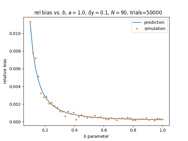
\ev{\hat{r}} \approx r \left( 1 + z_a^2 + z_b^2 \right)
$$
where $z_a \equiv \delta \tilde{y} / a$ and $z_b \equiv \delta \tilde{y} / b$.
We see that $\hat{R}$ ($\hat{r}$) is a biased estimator, though the bias is small provided $c_o,c_1$ ($a,b$) are much larger than $\delta \tilde{y}$.
To determine the variance or $\hat{R}$ we must evaluate the expectation value $\ev{\hat{R}^2} = \ev{\frac{|\hat{c}_1|^2}{\hat{c}_o^2}}$. Using the same taylor approximation this expression simplifies to
$$
\ev{\hat{R}^2} =
\ev{\frac{|\hat{c}_1|^2}{\hat{c}_o^2}} \approx
\frac{\ev{|\hat{c}_1|^2}}{\ev{\hat{c}_o^2}}\left( 1 + \frac{\text{var}\left(\hat{c}_o^2\right)}{\ev{\hat{c}_o^2}^2} \right)
$$
The only term remaining to calculate is $\ev{\hat{c}_o^4}$.
Like the four $\hat{\varepsilon}_i$ term in the $\ev{|c_1|^4}$ calculation, this term has no leading order contribution and so can be neglected.
For completeness we note that the calculation is identical to the one for $|\hat{c}_1|^4$ except all pairs contribute since the exponential term in the leading sum is reduced to $e^{i 2 \pi \left( 0 a + 0 b + 0 c + 0 d \right) / N} = 1$.
Totalling all the contributions gives us
$$
\ev{\hat{c}_o^4} = c_o^4 \left( 1 + 6 z_o^2 + 3 z_o^4 \right)
$$
or in other words
$$
\text{var}\left( \hat{c}_o^4 \right) = c_o^4 \left( 4 z_o^2 + 2 z_o^4 \right)
$$
so that
$$
\ev{\hat{R}^2} \approx
R^2 \frac{ 1 + z_1^2 }{ 1 + z_o^2 } \left( 1 + \frac{4 z_o^2 + 2 z_o^4}{1 + 2 z_o^2 + z_o^4} \right)
$$
Keeping only terms up to $z_n^2$ we get
$$
\ev{\hat{R}^2} \approx
R^2 \left( 1 + 3 z_o^2 + z_1^2 \right)
$$
So that
$$
\text{var}\left(\hat{R}\right) \approx
R^2 \left( z_o^2 + \frac{1}{2} z_1^2 \right)
$$
or
$$
\frac{\sigma_R}{R} \approx \sqrt{ z_o^2 + \frac{1}{2} z_1^2 }
$$
or
$$
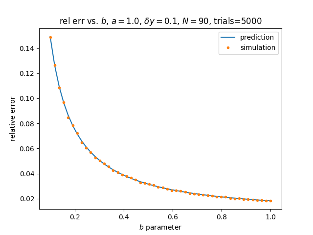
\frac{\sigma_r}{r} \approx \sqrt{ z_a^2 + 2 z_b^2 }
$$
Note that the (relative) bias is hardly worth correcting since it is smaller than the (relative) standard deviation by roughly a factor $\sqrt{ z_a^2 + z_b^2 }$.
Below are the results of some simulations to compare with our predictions
footnotes
1
To see this note that if $m = 0$ then
$$
\sum_{n=1}^N e^{i\frac{2 \pi m n}{N}} = \sum_{n=1}^N e^{i\frac{2 \pi (0) n}{N}} = \sum_{n=1}^N 1 = N
$$
If $m = 1,2,\ldots,N-1$ then $e^{i \frac{2 \pi M}{N}} \neq 1$ so we can apply the law for (finite) geometric series:
$$
\sum_{n=1}^N e^{i\frac{2 \pi M n}{N}} =
\frac{1 - e^{i 2\pi M}}{1 - e^{i \frac{2\pi M}{N}}} =
0
$$